This blog post is mostly motivated by the lack of comprehensive resources about variational inference found on internet. From my personal experience, resources are either too theoretical-oriented or turned to a too general audience. Both missing important stuff for my taste to allow researchers to implement their own models. In this first post on variational inference we will see how important results are derived from the theory, what is the intuition behind and how to implement the classical linear regression using variational inference by yourself. That being said, let’s start !
What is exactly Variational Inference ?
Variational inference (VI) is a family of methods, coming from the Machine Learning field, which approximates complex density functions. The main idea behind VI is to convert an estimation problem into an optimization one. VI is traditionally used in Bayesian inference , when the posterior density is intractable. I discovered the VI thanks to the wonderful works from the Stephens’ lab from Chicago or David Blei. However there applications for complex maximum likelihood estimations for frequentist models. During my research, I mostly played with variational inference for Bayesian models, i.e., variational bayes (VB). Thus, I will focus my attention on these latter, while applications of variational inference to frequentist models should be addressed in another post.
At the end of this tutorial, you will (hopefully) understand what is the variational bayes and how to implement it under the most common models encountered in practice.
Before going any further, a traditional variational bayes procedure needs:
- An intractable posterior to approximate
- A cost function to optimize over
- Procedure to find optimal parameters, e.g., which maximizes/minimizes the cost function
Why do we need variational inference in Bayesian models ?
Before answering this question, since I assume that many of you are not very familiar with Bayesian statistics let me start with the basics. What is exactly Bayesian inference and how is different from methods we use traditionally, e.g., frequentist methods?
In short, a typical Bayesian inference procedure considers the parameters as random variables and tries to estimate the posterior distribution of these parameters given the observed data. The former point is the central difference between Bayesian and frequentist methods. Indeed in frequentist frameworks, parameters are treated as fixed and the data as random. This gives us another angle for doing inferences with more intuitive interpretations than their frequentist counterparts (See my first post on the p-value: https://wordpress.com/post/statsxomics.blog/58). Formally the posterior can be obtained with the well-known Bayes’ theorem:

The numerator is formed by the product of the data likelihood and the prior over the parameters. In essence, Bayesian statistics are just a weighted version of the frequentist estimation, where the weight is the prior. Intuitively, if we have few data, the posterior will be driven by the prior, while large datasets will push the posterior to the data likelihood. The denominator (called the evidence or marginal) is obtained through a multi-dimensional numerical integration, which can be a daunting task to obtain, hence impossible in large dimensions.
To address this estimation problem, the most common strategy is to employ sampling procedures, such as Markov Chain Monte Carlo (MCMC) . While accurate, the procedure can be very slow, especially for large problems or non-conjugate models. This is where variational bayes procedures come into play.
Variational Bayes as an optimization problem
Instead of estimate the posterior through resampling, we can obtain it using optimization-based procedures. The core idea of a typical variational bayes procedure is to find a simple proxy distribution which approximates well the posterior. To do so, we have to find the proxy distribution (q) which minimizes the Kullback-Leibler divergence (DKL) with our target distribution (posterior). Formally:

Using few lines of standard algebra results, we can prove that the last quantity is always a function of the evidence (which is intractable).
Thus, instead of working directly with the DKL, we work with the well-known Evidence-Lower Bound (ELBO):


The right term of the last inequality corresponding to the ELBO formed by the full joint distribution (which is known) and the entropy of our optimal variational distributions. We will see later how to practically compute the ELBO.
Nonetheless, it remains few last steps before having a full procedure. Firstly, we have to assume a specific structure which links our proxy distributions together. The most common variational family is the mean-field factorization (all variational distributions q are independent), where each optimal variational distributions is governed by its own variational parameters. This is the factorization we will use.

We have not specified the parametric form but it will follow depending on the choice of prior in each model. Keep in mind that for a conjugate prior, the optimal variational distribution will have the same form as the prior under the mean-field factorization. After few lines of functional calculus, optimal variational distributions are obtained with:

In other words, this last equality tells us that the optimal variational distribution for a given parameter is independent of this parameter, but only depends on other variational parameters. This makes the use of EM-derived algorithms valid estimation procedures.
Then, we need a procedure which finds the best values for the variational parameters using the ELBO as cost function. Here I am focusing on Coordinate Ascent Variational Inference (CAVI) which is an iterative algorithm, updating the variational parameters successively.
Now we have reviewed important concepts underlying the VB, let’s make something concrete, applying the method to the Linear Regression.
Variational Bayes for a Linear Regression
A standard linear regression setup can defined by:


To summarize, what we are going to do is:
- Obtaining the functional form of optimal variational distributions for both
and
- Deriving the ELBO
- Implement CAVI in R for obtaining optimal variational parameters using the two previous steps
Optimal 
Only keeping the terms involving


which looks like an Inverse-Gamma distribution with its own variational parameters.

with


We will see in few seconds how to obtain 
Similarly for the 


This expression is the sum of two quadratics, by completing the square we obtain a Normal distribution with its own mean and variance parameters

where


Now we have all the variational parameters on which we will iterate over in the CAVI algorithm until the ELBO convergence. However, it remains some expectations that we want to compute. Using what we have just derived, the remaining expectations can be obtained using standard results:


Since all the optimal variational distributions have a closed-forms we can expressed the ELBO analytically:


where


For the sake of simplicity, the last expectation will be obtained using numerical integration.
Implementation in R
require(matrixcalc)
require(MCMCpack)

E_q_sigma2 = function(fn, alpha_sigma2,beta_sigma2) {
  integrate(function(sigma) {
    dinvgamma(sigma^2, shape = alpha_sigma2, scale = beta_sigma2) * fn(sigma)
  }, lower=0, upper= Inf)$value
}


entropy_sigma2 = function(alpha_sigma, beta_sigma){


  alpha_sigma+log(beta_sigma)+lgamma(alpha_sigma) - (1-alpha_sigma)*digamma(alpha_sigma)

}

entropy_lambda = function(alpha_lambda, beta_lambda){


  alpha_lambda+log(beta_lambda)+lgamma(alpha_lambda) - (1-alpha_lambda)*digamma(alpha_lambda)

}

entropy_beta = function(S,D){

  -0.5 * log(det(S)) - 0.5 * D * (1 + log(2*pi))
  #-0.5*(log(2*pi*sigma2_beta)+1)
}

lb_py=function(y,X,alpha_sigma2, beta_sigma2, mu_beta, sigma2_beta){
  #This function computes the lower bound for a linear regression with a gaussian y

  yy=crossprod(y,y)
  XX=crossprod(X,X)
  Xy=crossprod(X,y)

  mm = tcrossprod(mu_beta)
  E_q_log_sigma2 = E_q_sigma2(function(sigma) log(sigma^2), alpha_sigma2, beta_sigma2)
  E_q_log_inv_sigma2 = E_q_sigma2(function(sigma) log(1/sigma^2), alpha_sigma2, beta_sigma2)

  -0.5*(log(2*pi)+E_q_log_sigma2 + E_q_log_inv_sigma2 + yy + matrix.trace(XX%*%mm+sigma2_beta)-2*crossprod(mu_beta,Xy))
}


lb_pbeta = function(alpha_sigma2, beta_sigma2, mu_beta, sigma2_beta, tau2){
  E_q_log_sigma2 = E_q_sigma2(function(sigma) log(sigma^2), alpha_sigma2, beta_sigma2)

  mm = tcrossprod(mu_beta)

  -0.5*(log(2*pi)+sum(log(tau2))+E_q_log_sigma2+matrix.trace(mm+sigma2_beta)/(tau2+alpha_sigma2/beta_sigma2))
}

lb_psigma2=function(alpha_sigma2, beta_sigma2, prior="improper", alpha_0=0.001, beta_0=0.001){

  if(prior=="improper"){
    lb = E_q_sigma2(function(sigma) log(1/sigma^2), alpha_sigma2, beta_sigma2)
  } else if(prior=="inverse-gamma"){
    lb=alpha_0*log(beta_0)-lgamma(alpha_0)-(alpha_0+1)*(log(beta_sigma2)- digamma(alpha_sigma2))-beta_0/(alpha_sigma2/beta_sigma2)

  }
  lb

}


compute_ELBO=function(lb_py, lb_pbeta, lb_psigma2, entropy_sigma2, entropy_beta){
  lb = lb_py + lb_pbeta + lb_psigma2
  entropy = entropy_sigma2 + entropy_beta

  lb-entropy
}


lmcavi = function(y, X, sigma2_beta=1, tau2, nrep=1000, threshold=1e-6){
  #This function computes parameters of a multiple linear regression using variational Bayes
  #A multivariate gaussian is assumed for the prior over fixed effects
  #An improprer prior is assumed for the residual variance parameter

  list.result=list()

  n = length(y)
  p = ncol(X)

  XX=crossprod(X,X)
  Xy=crossprod(X,y)
  yy=crossprod(y,y)

  S = diag(sigma2_beta, p,p)

  alpha_sigma2 = (n+p)/2

  mu_beta = as.matrix(solve(XX + 1/tau2)%*%Xy, ncol=1) #if univariate: (sum_yx/(1/tau2 + sum_x2))

  mm = tcrossprod(mu_beta,mu_beta)
  A = yy+ matrix.trace(XX%*%(mm + S))  - 2*t(mu_beta)%*%Xy+ matrix.trace((mm + S)/tau2)#(sum_y2 + (mu_beta^2+sigma2_beta^2)*(sum_x2 + 1/tau2)-2*sum_yx*mu_beta)


  beta_sigma2 = (0.5*A)[1]
  sigma2_beta = solve((XX+1/tau2)%*%diag((alpha_sigma2/beta_sigma2)[1],p))

  lb_py = lb_py(y = y, X = X, mu_beta = mu_beta, sigma2_beta = sigma2_beta,alpha_sigma2 = alpha_sigma2 ,beta_sigma2 = beta_sigma2)
  lb_pbeta = lb_pbeta(alpha_sigma2,beta_sigma2, mu_beta, sigma2_beta, tau2)
  lb_psigma2 = lb_psigma2(alpha_sigma2,beta_sigma2)

  entropy_sigma2 = entropy_sigma2(alpha_sigma2,beta_sigma2)
  entropy_beta = entropy_beta(sigma2_beta, p)

  ELBO = compute_ELBO(lb_py, lb_pbeta, lb_psigma2, entropy_sigma2,  entropy_beta)


  list.result[["ELBO"]][1] = ELBO
  list.result[["mu_beta"]][[1]] = mu_beta
  list.result[["sigma2_beta"]][[1]] = sigma2_beta
  list.result[["alpha_sigma2"]][1] = alpha_sigma2
  list.result[["beta_sigma2"]][1] = beta_sigma2

  for(i in 2:nrep){
    print(i)
    S =   list.result[["sigma2_beta"]][[i-1]]

    A = yy+ matrix.trace(XX%*%(mm + S))  - 2*t(mu_beta)%*%Xy+ matrix.trace((mm + S)/tau2)#(sum_y2 + (mu_beta^2+sigma2_beta^2)*(sum_x2 + 1/tau2)-2*sum_yx*mu_beta)


    beta_sigma2 = (0.5*A)[1]
    sigma2_beta = solve((XX+1/tau2)%*%diag((alpha_sigma2/beta_sigma2)[1],p))

    lb_py = lb_py(y = y, X = X, alpha_sigma2 = alpha_sigma2, beta_sigma2 =  beta_sigma2, mu_beta = mu_beta, sigma2_beta = sigma2_beta)
    lb_pbeta = lb_pbeta(alpha_sigma2,beta_sigma2, mu_beta, sigma2_beta, tau2)
    lb_psigma2 = lb_psigma2(alpha_sigma2,beta_sigma2, prior = "inverse-gamma")

    entropy_sigma2 = entropy_sigma2(alpha_sigma2,beta_sigma2)
    entropy_beta = entropy_beta(sigma2_beta, p)

    ELBO = compute_ELBO(lb_py, lb_pbeta, lb_psigma2, entropy_sigma2,  entropy_beta)

    list.result[["ELBO"]][i] = ELBO
    list.result[["sigma2_beta"]][[i]] = sigma2_beta
    list.result[["beta_sigma2"]][i] = beta_sigma2

    if(abs(ELBO-list.result[["ELBO"]][i-1])<=threshold) break

  }

  structure(list.result, class="vblr")

}
Comparisons with MCMC: posterior and running times
Generating two toy datasets with 10 and 100 predictors for 1000 individuals we are able to compare with respect to the accuracy and running times the VB linear regression with the same model using MCMC. The code to reproduce the results is available at the end of this post.
| Scenario/Metrics | Bias | Running time (in seconds) |
| 1000 individuals – 10 predictors | 5.60e-05 | VB: 0.01 MCMC: 9.05 |
| 1000 individuals – 100 predictors | 6e-04 | VB: 0.22 MCMC: 23.87 |
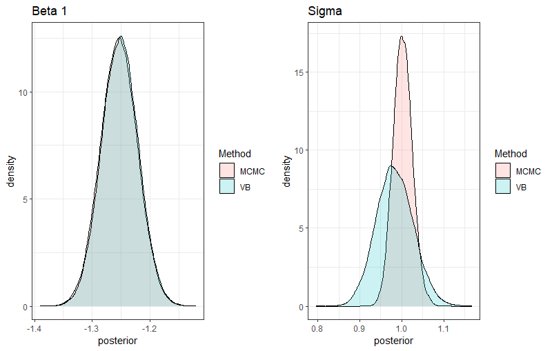
Interestingly, the CAVI algorithm converges in 6 iterations in the first scenario with 1000 individuals and 10 predictors and converges in 11 iterations in the second example with 100 predictors, providing very accurate estimations. Now if we compare the resulting posteriors in the first example for one beta and sigma obtained with VB compared to those estimated by MCMC, we observe a perfect adequation of the VB posterior for beta 1, while a slight discrepancy for sigma can be noted. Indeed, the MCMC retrieves the true value ( 

What Variational Bayes is and what is not ?
Ok now besides the technical aspects it remains important to understand when VB is a good option and when it’s not.
- VB is a good option when you are facing performance issues and you want to run models on large datasets. Even if few seconds is not a big deal, the differences in running time can be drastic for more complex problems.
- However if your problem is small with a simple model and a modest number of individuals or parameters, VB it is not worth the effort since it will require lot of mathematical derivations.
- VB is perfect for prediction, while for inferences it has to be applied with cautious. This is explained by the type of factorization used here (mean-field) which induces independency between the parameters, hence tends to underestimate the variance with over-optimistic inferences. Other types of factorization, such as structured VB, exists but require more advanced techniques.
Conclusion and general remarks
Finally, we have seen what is the mathematical steps for obtaining a VB model for linear regression and how to implement it in R. The cook recipe is quite long for such a simple model, with modest gains, but in more complex model like the logistic regression the gain could be exponential. I will cover this model in another post showing some strategies to work with non-conjugate models. Also, I did not discuss the different algorithms for optimizing the ELBO focusing on CAVI, gradient-based approaches are also available for these problems. Also, the ELBO is not a convex function and it is sensible to starting values, trying different values will lead to different optimal parameters. Finally, the most important thing here is that the computational gain is only possible by long mathematical derivations and homemade coding, since no R package implement this stuff. It exists however automatic VB approaches but they are not problem specific and cannot be well-suited for specific problems. I have started a project on Github for making available such techniques to a large audience: https://github.com/lmangnier/Variational_Bayes. Feel free to participate here or on my social platforms !
Let us render to Caesar what is Caesar’s, this post could not be possible without the two wonderful tutorials on which I drew lot of inspiration. Shoutout to https://rpubs.com/cakapourani/variational-bayes-lr and https://fabiandablander.com/r/Variational-Inference.html.
set.seed(1234)

gen_dat <- function(n,p ,beta, sigma) {
  X <- matrix(rnorm(n*p),nrow=n,ncol=p)
  y <- 0 + X%*%beta + rnorm(n, 0, sigma)
  data.frame(X = X, y = y)
}

beta1 = rnorm(10,0,1)
beta2 = rnorm(100,0,1)

datascenario1_1 = gen_dat(n = 1000,10,beta1,1 )
datascenario1_2 = gen_dat(n = 1000,100,beta2,1 )


lmcavi_scenario1_1 = lmcavi(as.matrix(datascenario1_1[,"y", drop=F]), as.matrix(datascenario1_1[,1:10]), tau2=0.5)


lmcavi_scenario1_2 = lmcavi(as.matrix(datascenario1_2[,"y", drop=F]), as.matrix(datascenario1_2[,1:100]), tau2=0.5)

model_lm_stan = "data {
  int<lower=0> n; //number of indidivuals
  vector[n] y; //vector of responses
  int<lower=0> K; //number of predictors
  matrix[n,K] X; //matrix of predictors
  real tau2;
}

parameters {
  vector[K] beta;
  real<lower=0> sigma;
}

model {
  target +=  -log(sigma);
  target += normal_lpdf(beta | 0, tau2*sigma);
  target += normal_lpdf(y | X*beta, sigma);
}"

stan_dat_1_1 = list('n' = nrow(datascenario1_1), "K" = 10,'X' = datascenario1_1[,-ncol(datascenario1_1)], 'y' = datascenario1_1[,ncol(datascenario1_1)], "tau2"=0.50)
stan_dat_1_2 = list('n' = nrow(datascenario1_2), "K" = 100,'X' = datascenario1_2[,-ncol(datascenario1_2)], 'y' = datascenario1_2[,ncol(datascenario1_2)], "tau2"=0.50)

fit1_1 = rstan::sampling(model_lm_stan, data = stan_dat_1_1, iter = 8000, refresh = FALSE, seed = 1)

fit1_2 = rstan::sampling(model_lm_stan , data = stan_dat_1_2, iter = 8000, refresh = FALSE, seed = 1)

Leave a comment