StatsXOmics

For everyone who has already built a machine learning model, there is no such consensus as: Building predictive model is not an easy task. Between the data cleaning and processing, the model learning, hyperparameter tuning, and post-hoc validation, there are too many choices that can hinder your model generalization and interpretability. With this in mind, feature selection has became on the most important part of any learning algorithm for limiting overfitting, improving result transferability.

From my classical background in statistics (a.k.a old fashioned stats), I really like one of family model which allows to automatically select features while predicting new values in an unified framework, the penalized regression. In this general class of models, you have one of its well-known member: the Least Absolute Shrinkage and Selection Operator, or LASSO. By penalizing model coefficients with a hyperparameter, the model can shrink parameters toward the mean value (0 in the case where the predictors have been centered), keeping only the most relevant features for your question. Besides the intuition, for purists like me, here the standard LASSO equation:

The first part is equivalent to the standard least squares while the right term is the penalty portion forcing coefficient to zeros. Lambda here is the shrinkage hyperparmater mentionned above. It is traditionally obtained using Cross-Validation. It exists alternatives or extensions to the LASSO, such as the ridge, elastic net or their Bayesian implementations for permitting feature selection with different goals in mind. For example, ridge cannot set coefficient exactly to zeros, while elastic net has better selection properties for highly correlated features. Importantly, penalized regressions are particularly useful for scenarios where the number of predictors are far greater the number of individuals or when the signal-to-noise ratio is particularly low, which can be assumed for many multi-omics problems.

However, for the reader aware of the issues induced by Cross-Validation, taking a different data partition will inevitably lead to a different set of selected features. So if my set of features is not stable across folds, how can I trust my model ? Left this way, it will be hard to tell whether your model identifies a true predictor or a false positive. This question paves the way for approaches like Stability Selection.

Based on this observation, two very clever statisticians, Meinshausen and Bühlmann in their paper proposed a powerful while easy implementable way to improve the LASSO, the Stability Selection (https://members.cbio.mines-paristech.fr/~jvert/svn/bibli/local/Meinshausen2010Stability.pdf). The idea behind Stability Selection is simple, instead of taking one repetition of data to build the LASSO, we can repeat the procedure many times (100 for instance) and establish the set of features kept a great portion of times. The great advantage is to not require of Cross-Validation, however it is more computational intensive. Stability Selection has incredible theoretical properties regarding Type-I error rate and empirically we will see in a short example that equivalent prediction performances are achieved with a smaller number of features. Here the general algorithm:

• Randomly select half the number of observations with no replacement
• Multiply the random predictor matrix by an uniformly distributed scaling factor between 0.2 and 0.8. Injecting random noise will help to stabilize the algorithm. This is referred as random LASSO.
• Fit the original LASSO on a pre-specified sequence of lambda with the scaled random predictors and outcome
• Create a binary matrix where a coefficient is 1 if its value is different from zero, 0 otherwise
• For each lamba, compute the proportion of the coefficient being nonzero across replicates
• Take the maximal proportion for each feature
• The feature is kept if and only if the maximal proportion is greater than a user-defined threshold (in practice between 0.5 and 0.8). All features kept are referred as stable set
• Finally, fit a model with only the stable set as predictors

As expected, you can play with the threshold parameter to keep more or less features depending on the research question. We will later see, that we are looking for some kind of trade-off between sparsity and predictive performance.

Illustration of stability selection in synthetic data

I generated 200 features following a centered and uncorrelated multivariate gaussian distribution. I randomly selected half the number of features to have a zero effect while the remaining portion have an effect following a gaussian distribution of mean = 10 and variance = 1.

Firstly, I ran a standard LASSO using the Cross-Validation for finding the relevant features. Interestingly, the model selected either 63 or 29 “significant” features depending on wheter the lambda.min (lambda reaching the minimal Mean Squared Error) or lambda.1se (most parcimonious model at 1 standard error of the minimal value) was used. Since we know the ground truth, I computed the proportion of non-zero features which are true non-null variables, 47% and 48% for each value of lambda, respectively.

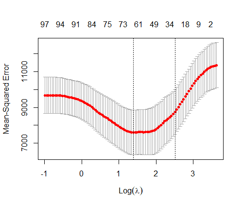
First observation, the model is relatively sparse. However, only half the detected “significant” features were found in the true set of features, which is not better as tossing a coin to tell if the variable is important or not. Regarding the predictive performance, using 10-folds CV, the standard LASSO exhibited a mean R2 of 0.35 (standard error = 0.29) and a mean R2 of 0.27 (standard error = 0.28), for lambda.min and lambda.1se, respectively, which is quite unstable depending on the fold considered.

We did the same thing using the Stability Selection algorithm shown above. The stability path below shows the Probability Selection for each feature across all lambdas. Red dottes lines correspond to the features where their maximal proportion is above 0.4.

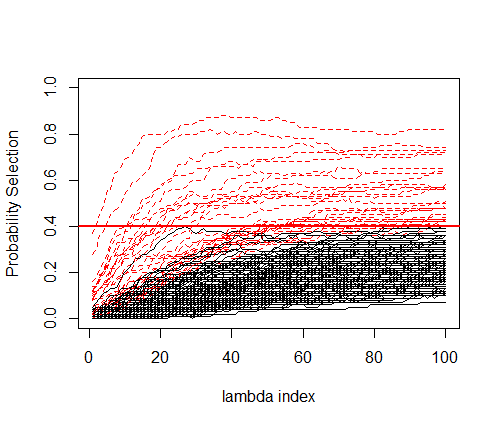
Interestingly, at the 0.4 threshold, 30 features were selectioned with 80% found in the true set of variables. That’s much higher than the original LASSO, suggesting that even if lot of features are not captured by the model the signal if of better quality. Now, an interesting thing to do is to compare the predictive performance of Stability Selection and compared it to what we have previously found. Using a 10folds-CV LASSO with Stability Selection showed equivalent predictive performances with a R2 of 0.32 (standard error = 0.27). We can now check if the algoritmns are stable regarding the number of features kept in the model across folds. On average, 23.3 features are kept using Stability Selection with a small variability (2.66), while regular LASSO gives 61.7 and 24.8 in both lambdas considered, with much higher variability (14.63; 17.35). Results were summarized below.

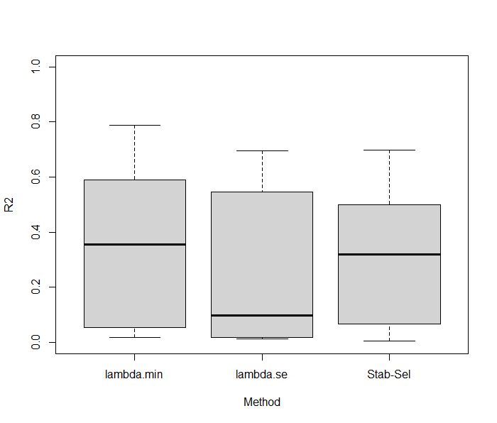
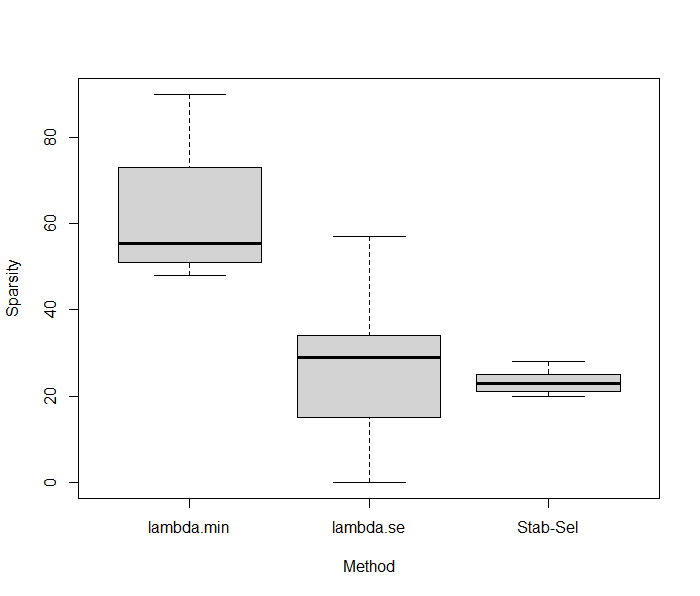
These results suggest that Stability Selection provides a powerful strategy for robust selection features with similar predictive performance results.

Stability Selection as a general procedure for feature selection for multi-omics data

We have seen that Stability Selection can improve the feature selection behavior of the LASSO. However, this is not the end of the story, the procedure can be used to any penalization-based method or as an automized strategy before putting the selected variables into a non-linear model such as random forest or kNN.

From a multi-omics perspective I argue that this kind of method can significantly enhance feature selection for multi-view approaches, like multi-view Lasso (https://cran.r-project.org/web/packages/multiview/vignettes/multiview.pdf), or multi-block sPLS(DA), since they represent efficient, while cost-reduced method for determining stable set of features. With critical improvement in result interpretability.

Recently, Hédou et al., in their paper proposed to combine Stability Selection with the knockoff to improve feature selection in high-dimensional multi-omics problems (https://www.nature.com/articles/s41587-023-02033-x). The paper is interesting in many different ways and is particularly relevant for people in the field.

As always, comments, questions, and suggestions are welcome.

library(glmnet) #For the LASSO

#'  A function for plotting stability path from the LASSO.SS function
#'  @param stability.scores a matrix as provided by LASSO.SS
#'  @param threshold a value between 0 and 1 corresponding to the threshold of the probability that the feature is kept across bootstraps
#'  @return a stability path plot
plot.LASSO.SS = function(stability.scores ,threshold=0.8){
  
  
  plot(1, type="n",ylim=c(0,1), xlim=c(1,100) ,xlab="lambda index", ylab="Probability Selection")
  
  
  max.by.features = apply(stability.scores,1,max)
  
  for(i in 1:nrow(stability.scores)) {
    
    if(max.by.features[i] > threshold) lines(1:ncol(stability.scores),stability.scores[i,], col="red", lty=2) 
    else lines(1:ncol(stability.scores),stability.scores[i,])
    
  }
  abline(h=threshold, lwd=2, col="red")
}

set.seed(1234)

#Generating synthetic data
X = MASS::mvrnorm(100, mu=rnorm(200), Sigma = diag(1,200))
colnames(X)=paste0("Var",1:200)
beta = rnorm(ncol(X), 10)
prop.zeros = 0.5

index.zeros = sample(ncol(X), ncol(X)*prop.zeros)
beta[index.zeros] = 0



y = 0.8 + X%*%beta + rnorm(100)

#Original LASSO
m=cv.glmnet(X, y)

plot(m)

#Number of features selected by the model whic are true positives for the LASSO
sum((which(as.matrix(coef(m, s="lambda.min"))[-1,]!=0)+1) %in% which(beta!=0)) / length(which(as.matrix(coef(m, s="lambda.min"))[-1,]!=0))
sum((which(as.matrix(coef(m, s="lambda.1se"))[-1,]!=0)+1) %in% which(beta!=0)) / length(which(as.matrix(coef(m, s="lambda.1se"))[-1,]!=0))
length(which(as.matrix(coef(m, s="lambda.min"))[-1,]!=0))
length(which(as.matrix(coef(m, s="lambda.1se"))[-1,]!=0))

##Stability Selection on the full dataset
n=nrow(X); p=ncol(X)
coefs.boots = list()
for(i in 1:100){
  random.index = sample(1:n, 0.5*n, replace = FALSE)
  
  X.sub = X[random.index,]
  y.sub = y[random.index]
  
  #Randomized LASSO
  scaling_factors = runif(p, 0.2,0.8)
  X.random = X.sub*scaling_factors
  
  fit = glmnet(X.random, y.sub, alpha = 1, lambda=m$lambda, family = "gaussian",standardize = TRUE) 
  #lambda sequence is specified by hand 
  
  coefs=as.matrix(coef(fit))[-1,]
  coefs[coefs!=0] = 1
  
  coefs.boots[[i]]=coefs
}


stability.scores = Reduce("+", coefs.boots)/100

plot.LASSO.SS(stability.scores, threshold = 0.4)
max.by.features = apply(stability.scores, 1, max)

#Number of features selected by the model whic are true positives for the Stability Selection
length(which(max.by.features>=0.4))
sum(which(max.by.features>=0.4) %in% which(beta!=0))/length(which(max.by.features>=0.4))


fold=sample(1:10, nrow(X), replace=T)

X.folds = cbind(fold,X)

R2.CV.LASSO.SS = list()
R2.CV.LASSO = list()

sparsity.CV.LASSO.SS = list()
sparsity.CV.LASSO = list()

for(f in unique(fold)){
  
  coefs.boots = list()
  
  X.test = X.folds[fold==f,]
  X.train = X.folds[fold!=f,]
  
  y.test = y[fold==f,,drop=F]
  y.train = y[fold!=f,,drop=F]
  
  
  glmnetcv = cv.glmnet(X.train, y.train)
  
  
  pred.min = predict(glmnetcv, X.test, s="lambda.min")
  pred.1se = predict(glmnetcv, X.test, s="lambda.1se")
  
  nzeros.min = length(which(as.matrix(coef(glmnetcv, s="lambda.min")[-1,])!=0))
  nzeros.1se = length(which(as.matrix(coef(glmnetcv, s="lambda.1se")[-1,])!=0))
  
  pred = cbind(pred.min, pred.1se)
  R2.CV.LASSO[[f]] = apply(pred, 2, function(x) cor(x, y.test)^2)
  sparsity.CV.LASSO[[f]] = c(nzeros.min, nzeros.1se)
  
  n=nrow(X.train); p=ncol(X.train)
  
  for(i in 1:100){
    random.index = sample(1:n, 0.5*n, replace = FALSE)
    
    X.sub = X.train[random.index,]
    y.sub = y.train[random.index, ,drop=F]
    
    #Randomized LASSO
    scaling_factors = runif(p, 0.2,0.8)
    X.random = X.sub*scaling_factors
    
    fit = glmnet(X.random, y.sub, alpha = 1, lambda=m$lambda, family = "gaussian",standardize = TRUE) 
    #lambda sequence is specified by hand 
    
    coefs=as.matrix(coef(fit))[-1,]
    coefs[coefs!=0] = 1
    
    coefs.boots[[i]]=coefs
  }
  stability.scores = Reduce("+", coefs.boots)/100
  max.by.features = apply(stability.scores, 1, max)
  
  kept.features = which(max.by.features>=0.4)
  X.train.subset = X.train[,kept.features]
  
  df.y.X.train.subset = data.frame(X.train.subset, "y"=y.train)
  
  model=lm(y~., df.y.X.train.subset)

  pred = predict(model,as.data.frame(X.test[, kept.features]))
  
  sparsity.CV.LASSO.SS[[f]] = length(kept.features)
  R2.CV.LASSO.SS[[f]] = cor(pred, y.test)^2
  
}

#Results across 10folds-CV
mean(unlist(results.CV.LASSO.SS)); sd(unlist(results.CV.LASSO.SS))
mean(unlist(sparsity.CV.LASSO.SS));sd(unlist(sparsity.CV.LASSO.SS))

apply(do.call("rbind",results.CV.LASSO), 2, mean, na.rm=TRUE)
apply(do.call("rbind",results.CV.LASSO), 2, sd,na.rm=TRUE)

apply(do.call("rbind",sparsity.CV.LASSO), 2, mean, na.rm=TRUE)
apply(do.call("rbind",sparsity.CV.LASSO), 2, sd,na.rm=TRUE)


boxplot(cbind(do.call("rbind",results.CV.LASSO), unlist(results.CV.LASSO.SS)), names=c("lambda.min", "lambda.se", "Stab-Sel"), ylim=c(0,1), xlab="Method", ylab="R2")
boxplot(cbind(do.call("rbind",sparsity.CV.LASSO), unlist(sparsity.CV.LASSO.SS)), names=c("lambda.min", "lambda.se", "Stab-Sel"), xlab="Method", ylab="Sparsity")